Data Structure and Types

A Data Structure delivers a structured set of variables related to each other in various ways. It forms the basis of a programming tool that signifies the relationship between the data elements and allows programmers to process the data efficiently.

We can classify Data Structures into two categories:

Primitive Data Structure
Non-Primitive Data Structure

The following figure shows the different classifications of Data Structures.

Primitive Data Structures

Primitive Data Structures are the data structures consisting of the numbers and the characters that come in-built into programs.

These data structures can be manipulated or operated directly by machine-level instructions.

Basic data types like Integer, Float, Character, and Boolean come under the Primitive Data Structures.

These data types are also called Simple data types, as they contain characters that can't be divided further.

Non-Primitive Data Structures

Non-Primitive Data Structures are those data structures derived from Primitive Data Structures.

These data structures can't be manipulated or operated directly by machine-level instructions.

The focus of these data structures is on forming a set of data elements that is either homogeneous (same data type) or heterogeneous (different data types).

Based on the structure and arrangement of data, we can divide these data structures into two sub-categories -

Linear Data Structures
Non-Linear Data Structures

Linear Data Structures

A data structure that preserves a linear connection among its data elements is known as a Linear Data Structure. The arrangement of the data is done linearly, where each element consists of the successors and predecessors except the first and the last data element. However, it is not necessarily true in the case of memory, as the arrangement may not be sequential.

Based on memory allocation, the Linear Data Structures are further classified into two types:

Static Data Structures:

The data structures having a fixed size are known as Static Data Structures. The memory for these data structures is allocated at the compiler time, and their size cannot be changed by the user after being compiled; however, the data stored in them can be altered. The

Array is the best example of the Static Data Structure as they have a fixed size, and its data can be modified later.

Dynamic Data Structures:

The data structures having a dynamic size are known as Dynamic Data Structures. The memory of these data structures is allocated at the run time, and their size varies during the run time of the code. Moreover, the user can change the size as well as the data elements stored in these data structures at the run time of the code.

Linked Lists, Stacks, and Queues are common examples of dynamic data structures.

Types of Linear Data Structures are:

The following is the list of Linear Data Structures that we generally use:

1. Arrays

An Array is a data structure used to collect multiple data elements of the same data type into one variable. Instead of storing multiple values of the same data types in separate variable names, we could store all of them together into one variable. This statement doesn't imply that we will have to unite all the values of the same data type in any program into one array of that data type.

But there will often be times when some specific variables of the same data types are all related to one another in a way appropriate for an array.

An Array is a list of elements where each element has a unique place in the list. The data elements of the array share the same variable name; however, each carries a different index number called a subscript. We can access any data element from the list with the help of its location in the list.

Thus, the key feature of the arrays to understand is that the data is stored in contiguous memory locations, making it possible for the users to traverse through the data elements of the array using their respective indexes.

Arrays can be classified into different types:

One-Dimensional Array: An Array with only one row of data elements is known as a One-Dimensional Array. It is stored in ascending storage location.
Two-Dimensional Array: An Array consisting of multiple rows and columns of data elements is called a Two-Dimensional Array. It is also known as a Matrix.
Multidimensional Array: We can define Multidimensional Array as an Array of Arrays. Multidimensional Arrays are not bounded to two indices or two dimensions as they can include as many indices are per the need.

2. Linked Lists

A Linked List is another example of a linear data structure used to store a collection of data elements dynamically. Data elements in this data structure are represented by the Nodes, connected using links or pointers.

Each node contains two fields, the information field consists of the actual data, and the pointer field consists of the address of the subsequent nodes in the list.

The pointer of the last node of the linked list consists of a null pointer, as it points to nothing. Unlike the Arrays, the user can dynamically adjust the size of a Linked List as per the requirements.

Linked Lists can be classified into different types:

Singly Linked List: A Singly Linked List is the most common type of Linked List. Each node has data and a pointer field containing an address to the next node.
Doubly Linked List: A Doubly Linked List consists of an information field and two pointer fields. The information field contains the data. The first pointer field contains an address of the previous node, whereas another pointer field contains a reference to the next node. Thus, we can go in both directions (backward as well as forward).
Circular Linked List: The Circular Linked List is similar to the Singly Linked List. The only key difference is that the last node contains the address of the first node, forming a circular loop in the Circular Linked List.

3. Stacks

A Stack is a Linear Data Structure that follows the LIFO (Last In, First Out) principle that allows operations like insertion and deletion from one end of the Stack, i.e., Top.

Stacks can be implemented with the help of contiguous memory, an Array, and non-contiguous memory, a Linked List. Real-life examples of Stacks are piles of books, a deck of cards, piles of money, and many more.

The primary operations in the Stack are as follows:

Push: Operation to insert a new element in the Stack is termed as Push Operation.
Pop: Operation to remove or delete elements from the Stack is termed as Pop Operation.

In a stack, operations can be perform only from one end (top here).

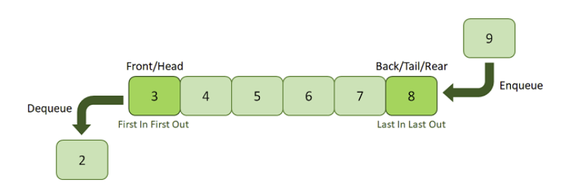
4. Queues

A Queue is a linear data structure similar to a Stack with some limitations on the insertion and deletion of the elements. The insertion of an element in a Queue is done at one end, and the removal is done at another or opposite end.

Thus, we can conclude that the Queue data structure follows FIFO (First In, First Out) principle to manipulate the data elements. Implementation of Queues can be done using Arrays, Linked Lists, or Stacks.

Some real-life examples of Queues are a line at the ticket counter, an escalator, a car wash, and many more.

The following are the primary operations of the Queue:

Enqueue: The insertion or Addition of some data elements to the Queue is called Enqueue. The element insertion is always done with the help of the rear pointer.
Dequeue: Deleting or removing data elements from the Queue is termed Dequeue. The deletion of the element is always done with the help of the front pointer.

Non-Linear Data Structures

Non-Linear Data Structures are data structures where the data elements are not arranged in sequential order. Here, the insertion and removal of data are not feasible in a linear manner. There exists a hierarchical relationship between the individual data items.

The following types of Non-Linear Data Structures that we generally use:

1. Trees

A Tree is a Non-Linear Data Structure and a hierarchy containing a collection of nodes such that each node of the tree stores a value and a list of references to other nodes (the "children").

The Tree data structure is a specialized method to arrange and collect data in the computer to be utilized more effectively. It contains a central node, structural nodes, and sub-nodes connected via edges. We can also say that the tree data structure consists of roots, branches, and leaves connected.

Trees can be classified into different types:

Binary Tree: A Tree data structure where each parent node can have at most two children is termed a Binary Tree.
Binary Search Tree: A Binary Search Tree is a Tree data structure where we can easily maintain a sorted list of numbers.
AVL Tree: An AVL Tree is a self-balancing Binary Search Tree where each node maintains extra information known as a Balance Factor whose value is either -1, 0, or +1.
B-Tree: A B-Tree is a special type of self-balancing Binary Search Tree where each node consists of multiple keys and can have more than two children.

2. Graphs

A Graph is another example of a Non-Linear Data Structure comprising a finite number of nodes or vertices and the edges connecting them. The Graphs are utilized to address problems of the real world in which it denotes the problem area as a network such as social networks, circuit networks, and telephone networks.

For instance, the nodes or vertices of a Graph can represent a single user in a telephone network, while the edges represent the link between them via telephone.

The Graph data structure, G is considered a mathematical structure comprised of a set of vertices, V and a set of edges, E as shown below:

G = (V,E)

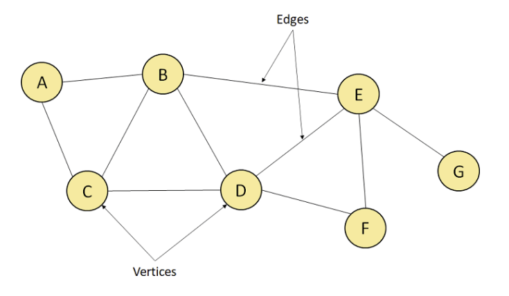
The above figure represents a Graph having seven vertices A, B, C, D, E, F, G, and ten edges [A, B], [A, C], [B, C], [B, D], [B, E], [C, D], [D, E], [D, F], [E, F], and [E, G].

Depending upon the position of the vertices and edges, the Graphs can be classified into different types:

Null Graph: A Graph with an empty set of edges is termed a Null Graph.
Trivial Graph: A Graph having only one vertex is termed a Trivial Graph.
Simple Graph: A Graph with neither self-loops nor multiple edges is known as a Simple Graph.
Multi Graph: A Graph is said to be Multi if it consists of multiple edges but no self loops.
Pseudo Graph: A Graph with self-loops and multiple edges is termed a Pseudo Graph.
Non-Directed Graph: A Graph consisting of non-directed edges is known as a Non Directed Graph.
Directed Graph: A Graph consisting of the directed edges between the vertices is known as a Directed Graph.
Connected Graph: A Graph with at least a single path between every pair of vertices is termed a Connected Graph.
Disconnected Graph: A Graph where there does not exist any path between at least one pair of vertices is termed a Disconnected Graph.
Regular Graph: A Graph where all vertices have the same degree is termed a Regular Graph.
Complete Graph: A Graph in which all vertices have an edge between every pair of vertices is known as a Complete Graph.
Cycle Graph: A Graph is said to be a Cycle if it has at least three vertices and edges that form a cycle.
Cyclic Graph: A Graph is said to be Cyclic if and only if at least one cycle exists.
Acyclic Graph: A Graph having zero cycles is termed an Acyclic Graph.
Finite Graph: A Graph with a finite number of vertices and edges is known as a Finite Graph.
Infinite Graph: A Graph with an infinite number of vertices and edges is known as an Infinite Graph.
Bipartite Graph: A Graph where the vertices can be divided into independent sets A and B, and all the vertices of set A should only be connected to the vertices present in set B with some edges is termed a Bipartite Graph.
Planar Graph: A Graph is said to be a Planar if we can draw it in a single plane with two edges intersecting each other.
Euler Graph: A Graph is said to be Euler if and only if all the vertices are even degrees.
Hamiltonian Graph: A Connected Graph consisting of a Hamiltonian circuit is known as a Hamiltonian Graph.

Graphs help us represent routes and networks in transportation, travel, and communication applications. And also help us represent the interconnections in social networks and other network-based applications.

Menu